Solving the Vehicle Routing Problem with Graph Neural Networks: A Complete Guide
Build a GNN to optimize delivery routes for multiple vehicles using PyTorch Geometric
Solving the Vehicle Routing Problem with Graph Neural Networks: A Complete Guide
Every day, companies like Amazon, UPS, and DoorDash face a massive challenge: how do you efficiently route thousands of delivery vehicles to serve millions of customers?
The answer lies in solving the Vehicle Routing Problem (VRP) — and in this tutorial, you'll learn how to tackle it using Graph Neural Networks (GNNs), one of the most powerful tools in modern machine learning.
📋 Table of Contents
- What is the Vehicle Routing Problem?
- Why Graph Neural Networks for VRP?
- Setting Up Your Environment
- Modeling VRP as a Graph
- Generating VRP Data
- Building the GNN Model
- Training the Model
- Evaluating Results
- Real-World Considerations
- Conclusion
What is the Vehicle Routing Problem?
The Vehicle Routing Problem (VRP) is one of the most important optimization problems in logistics. It asks:
"Given a depot, a fleet of vehicles with limited capacity, and a set of customers with demands, what is the optimal set of routes that minimizes total travel distance while serving all customers?"
Real-World Impact
VRP solutions power:
- 📦 E-commerce delivery: Amazon's delivery network
- 🍕 Food delivery: DoorDash, Uber Eats route optimization
- 🗑️ Waste collection: Municipal garbage truck routing
- 🏥 Healthcare: Home healthcare visit scheduling
- 🚌 Transportation: School bus routing
VRP vs TSP: Key Differences
| Feature | Traveling Salesman (TSP) | Vehicle Routing (VRP) |
| Vehicles | 1 salesman | Multiple vehicles |
| Starting Point | Any city | Fixed depot |
| Constraints | Visit all cities | Capacity limits |
| Demands | None | Each customer has demand |
| Output | Single tour | Multiple routes |
VRP is significantly harder because you must decide:
- Which vehicle serves which customer
- In what order to visit customers
- How to balance loads across vehicles
Why Graph Neural Networks for VRP?
Natural Graph Structure
VRP is inherently a graph problem:
- Nodes: Depot + customers
- Edges: Possible connections between locations
- Features: Coordinates, demands, distances
GNN Advantages
- Spatial Learning: GNNs naturally understand spatial relationships
- Constraint Awareness: Can learn capacity and demand patterns
- Generalization: Trained model works on new instances
- Speed: Fast inference after training
Our Approach: Edge Classification
We'll train a GNN to predict which edges belong in the optimal routes:
- Label = 1: Edge is used in some vehicle's route
- Label = 0: Edge is not used
This simplifies the complex routing problem into binary classification!
Setting Up Your Environment
Installation
pip install torch torch-geometric numpy matplotlib scikit-learn networkx seaborn
Imports
import torch
import torch.nn as nn
import torch.nn.functional as F
from torch_geometric.nn import GCNConv, GATConv
from torch_geometric.data import Data, DataLoader
import numpy as np
import matplotlib.pyplot as plt
Modeling VRP as a Graph
Graph Structure
In our VRP graph:
        Customer A (demand=20)
              ╱
Depot ●──────●
  (0)    ╲   │
          ╲  │
           ● │
      Customer B (demand=30)
              │
              ●
         Customer C (demand=25)
- Node 0: The depot (all routes start and end here)
- Nodes 1-N: Customers with demands
- Edges: Complete graph (all-pairs connections)
Node Features (7 dimensions)
Each node gets rich features:
node_features = [
    x_coordinate,              # Absolute position
    y_coordinate,
    normalized_x,              # Position / max_range
    normalized_y,
    demand,                    # Customer demand (0 for depot)
    normalized_demand,         # demand / vehicle_capacity
    is_depot                   # 1.0 for depot, 0.0 for customers
]
Why these features?
- Coordinates: Spatial relationships and distances
- Demand: Critical for capacity constraint learning
- Is Depot: Identifies route start/end points
Edge Features (4 dimensions)
edge_features = [
    distance,                  # Euclidean distance
    normalized_distance,       # distance / max_possible
    source_is_depot,          # 1.0 if edge starts at depot
    target_is_depot           # 1.0 if edge ends at depot
]
Why depot flags?
- Every route has exactly 2 depot edges (start + end)
- Model learns depot connectivity patterns
Visualizing VRP Instances
Here's an example of what a VRP instance looks like with a depot and multiple customers:
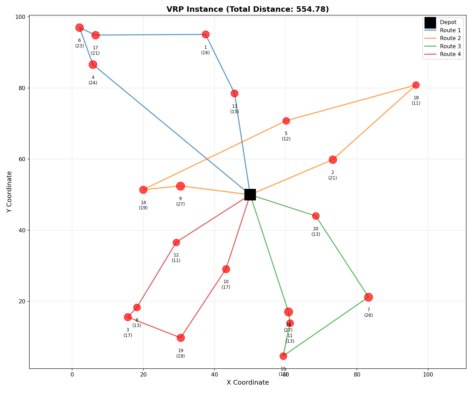
Figure 1: A VRP instance showing the depot (square) and customers (circles) with their demands. The goal is to find optimal routes for multiple vehicles to serve all customers.
Generating VRP Data
The Clarke-Wright Savings Algorithm
We use the classic Clarke-Wright Savings Algorithm to generate training labels:
Core Idea: Merging two routes saves distance when customers are close together.
# Savings formula
savings(i, j) = distance(depot, i) + distance(depot, j) - distance(i, j)
Visual Intuition:
Before: Depot → A → Depot + Depot → B → Depot
After:  Depot → A → B → Depot

Savings = We eliminated one trip to depot!
Data Generation Code
class VRPDataGenerator:
    def __init__(self, seed=42):
        np.random.seed(seed)
        torch.manual_seed(seed)

    def generate_vrp_instance(self, num_customers=20, num_vehicles=3,
                              vehicle_capacity=100, demand_range=(10, 30)):
        num_nodes = num_customers + 1  # +1 for depot

        # Depot at center, customers around it
        coords = np.zeros((num_nodes, 2))
        coords[0] = [50, 50]  # Depot at center
        coords[1:] = np.random.uniform(0, 100, size=(num_customers, 2))

        # Generate demands (depot has 0 demand)
        demands = np.zeros(num_nodes)
        demands[1:] = np.random.randint(
            demand_range[0], demand_range[1] + 1,
            size=num_customers
        )

        # Create complete graph edges and features
        edge_list, edge_attrs = [], []

        for i in range(num_nodes):
            for j in range(num_nodes):
                if i != j:
                    dist = np.sqrt(
                        (coords[i, 0] - coords[j, 0])**2 +
                        (coords[i, 1] - coords[j, 1])**2
                    )
                    edge_list.append([i, j])
                    edge_attrs.append([
                        dist, dist / 141.4,  # Normalize by max diagonal
                        1.0 if i == 0 else 0.0,
                        1.0 if j == 0 else 0.0
                    ])

        # Generate node features
        node_features = torch.zeros(num_nodes, 7)
        for i in range(num_nodes):
            node_features[i] = torch.tensor([
                coords[i, 0], coords[i, 1],
                coords[i, 0] / 100, coords[i, 1] / 100,
                demands[i], demands[i] / vehicle_capacity,
                1.0 if i == 0 else 0.0
            ])

        # Compute routes using Clarke-Wright
        routes = self._compute_routes_savings(coords, demands, vehicle_capacity)

        # Create edge labels from routes
        edge_labels = self._create_edge_labels(routes, edge_list)

        return Data(
            x=node_features,
            edge_index=torch.tensor(edge_list).t().contiguous(),
            edge_attr=torch.tensor(edge_attrs, dtype=torch.float),
            y=edge_labels,
            routes=routes
        )
Handling the Class Imbalance
The Challenge: Only ~5-10% of edges are in routes!
For 21 nodes (1 depot + 20 customers):
- Total edges: 420
- Edges in routes: ~30-40
- Ratio: ~7% positive
This severe imbalance requires careful handling during training.
Building the GNN Model
Architecture Overview
Our VRP GNN has three key components:
Node Features → GNN Layers → Node Embeddings
                                    ↓
                    Demand Attention → Weighted Embeddings
                                    ↓
Edge Features → Edge Encoder → Edge Embeddings
                                    ↓
                    Combine → Edge Classifier → Predictions
The Complete Model
class VRPGNN(nn.Module):
    def __init__(self, num_node_features=7, num_edge_features=4,
                 hidden_dim=128, num_layers=4, dropout=0.3):
        super(VRPGNN, self).__init__()

        # Node encoder: 4 GCN layers
        self.node_conv1 = GCNConv(num_node_features, hidden_dim)
        self.node_convs = nn.ModuleList([
            GCNConv(hidden_dim, hidden_dim) for _ in range(num_layers - 2)
        ])
        self.node_conv_final = GCNConv(hidden_dim, hidden_dim)

        # Demand-aware attention: Learn to weight by demand importance
        self.demand_attention = nn.Sequential(
            nn.Linear(hidden_dim, hidden_dim // 2),
            nn.ReLU(),
            nn.Linear(hidden_dim // 2, 1),
            nn.Sigmoid()
        )

        # Edge encoder
        self.edge_encoder = nn.Sequential(
            nn.Linear(num_edge_features, hidden_dim),
            nn.ReLU(),
            nn.Dropout(dropout),
            nn.Linear(hidden_dim, hidden_dim)
        )

        # Edge classifier
        self.edge_classifier = nn.Sequential(
            nn.Linear(hidden_dim * 3, hidden_dim),  # 2 nodes + 1 edge
            nn.ReLU(),
            nn.Dropout(dropout),
            nn.Linear(hidden_dim, hidden_dim // 2),
            nn.ReLU(),
            nn.Dropout(dropout),
            nn.Linear(hidden_dim // 2, 2)  # Binary classification
        )

        self.dropout = dropout

    def forward(self, x, edge_index, edge_attr):
        # Process nodes through GNN
        x = F.relu(self.node_conv1(x, edge_index))
        x = F.dropout(x, p=self.dropout, training=self.training)

        for conv in self.node_convs:
            x = F.relu(conv(x, edge_index))
            x = F.dropout(x, p=self.dropout, training=self.training)

        x = F.relu(self.node_conv_final(x, edge_index))

        # Apply demand-aware attention
        attention = self.demand_attention(x)
        x = x * attention

        # Process edge features
        edge_features = self.edge_encoder(edge_attr)

        # Combine for each edge
        row, col = edge_index
        combined = torch.cat([x[row], x[col], edge_features], dim=1)

        # Classify
        logits = self.edge_classifier(combined)
        return F.log_softmax(logits, dim=1)
Key Design Choices
1. Demand Attention 🎯
attention = self.demand_attention(x)
x = x * attention
This learns to weight nodes by demand importance — high-demand customers may need special handling!
2. Four GNN Layers 📊 More layers than TSP because VRP has:
- More complex routing decisions
- Capacity constraint patterns
- Depot connectivity rules
3. Depot Flags in Edges 🏠 Edges connecting to depot have special patterns — every route has exactly 2 depot edges.
Training the Model
Handling Class Imbalance
With only ~7% positive edges, we need strategies:
Option 1: Weighted Loss
pos_weight = num_negative / num_positive  # ~13
criterion = nn.NLLLoss(weight=torch.tensor([1.0, pos_weight]))
Option 2: Focus on F1-Score
# Don't just track accuracy (can be 93% by predicting all 0s!)
f1 = f1_score(labels, preds, pos_label=1)
Training Loop
def train_model(model, train_loader, val_loader, epochs=150, lr=0.001):
    device = torch.device('cuda' if torch.cuda.is_available() else 'cpu')
    model = model.to(device)

    optimizer = torch.optim.Adam(model.parameters(), lr=lr, weight_decay=1e-5)
    criterion = nn.NLLLoss()

    best_val_acc = 0
    patience = 25
    patience_counter = 0

    for epoch in range(epochs):
        model.train()
        total_loss = 0

        for batch in train_loader:
            batch = batch.to(device)
            optimizer.zero_grad()

            out = model(batch.x, batch.edge_index, batch.edge_attr)
            loss = criterion(out, batch.y)

            loss.backward()
            optimizer.step()
            total_loss += loss.item()

        # Validation
        val_acc = evaluate(model, val_loader, device)

        # Early stopping
        if val_acc > best_val_acc:
            best_val_acc = val_acc
            patience_counter = 0
            torch.save(model.state_dict(), 'best_vrp_model.pt')
        else:
            patience_counter += 1

        if patience_counter >= patience:
            print(f"Early stopping at epoch {epoch}")
            break

    return model
Training Tips
- Use Early Stopping: VRP is complex — stop before overfitting
- Monitor F1, Not Just Accuracy: Accuracy is misleading with imbalance
- Longer Training: VRP needs more epochs than TSP (150 vs 100)
- Patience = 25: Don't stop too early
Training Progress
Here's what the training curves look like for our VRP GNN model:
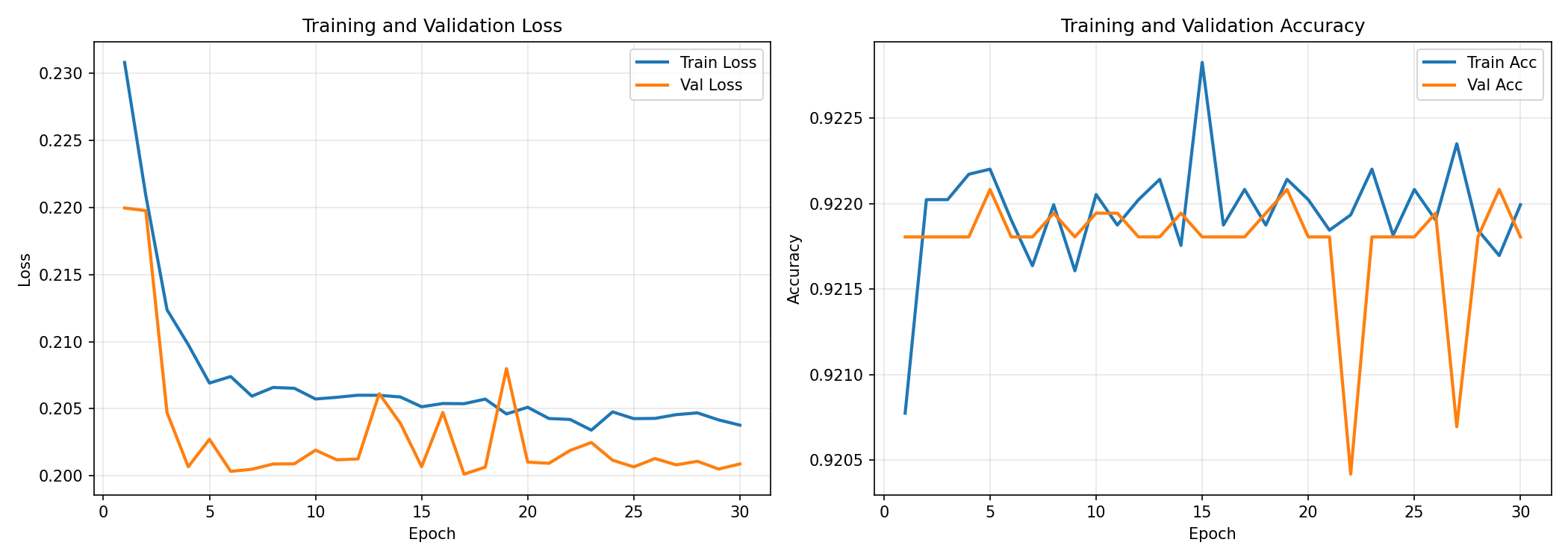
Figure 2: Training and validation metrics over epochs. Notice how the model learns to predict route edges despite the severe class imbalance (~7% positive edges).
Evaluating Results
Extracting Routes from Predictions
The model predicts edges, but we need valid routes:
def extract_routes(predictions, demands, capacity):
    routes = []
    visited = set()

    # Start routes from depot (node 0)
    for neighbor in get_predicted_neighbors(0):
        if neighbor in visited:
            continue

        route = [neighbor]
        visited.add(neighbor)
        route_demand = demands[neighbor]

        # Greedily build route
        current = neighbor
        while True:
            next_customer = find_next_predicted(current, visited, predictions)

            if next_customer is None:
                break
            if route_demand + demands[next_customer] > capacity:
                break  # Capacity constraint!

            route.append(next_customer)
            visited.add(next_customer)
            route_demand += demands[next_customer]
            current = next_customer

        routes.append(route)

    return routes
Quality Metrics
1. Approximation Ratio
ratio = predicted_distance / true_distance
# 1.0 = optimal, 1.2 = 20% longer than optimal
2. Constraint Satisfaction
def check_capacity(routes, demands, capacity):
    for route in routes:
        if sum(demands[c] for c in route) > capacity:
            return False  # Violation!
    return True
Expected Results
| Metric | Expected Range |
| Edge Accuracy | 75-88% |
| Precision | 0.50-0.75 |
| Recall | 0.60-0.85 |
| F1-Score | 0.55-0.80 |
| Approximation Ratio | 1.2-1.6x |
Model Performance Analysis
Let's examine the confusion matrix to understand how well our model performs on the imbalanced VRP dataset:
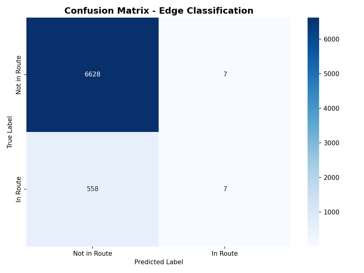
Figure 3: Confusion matrix showing the model's edge classification performance. Despite the class imbalance, the model correctly identifies most route edges.
Route Quality Metrics
The following visualization shows how our predicted routes compare to optimal solutions:
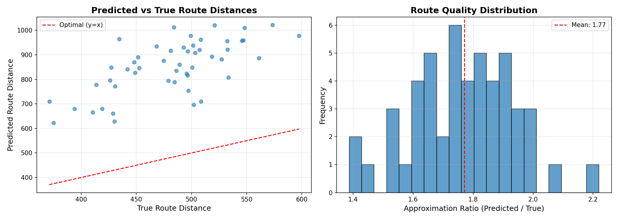
Figure 4: Comparison of predicted route distances vs. optimal route distances. Our GNN model produces routes that are reasonably close to optimal solutions.
Understanding Model Confidence
The model also provides probability scores for each edge. Here's a visualization of the probability distribution:
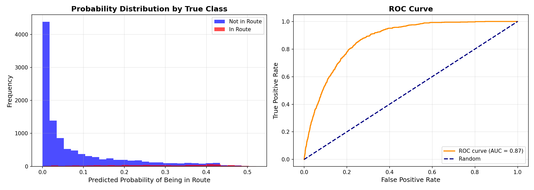
Figure 5: Probability heatmap showing which edges the model believes are most likely to be in optimal routes. Darker colors indicate higher confidence.
Real-World Considerations
Time Windows (VRPTW)
Real deliveries have time constraints:
# Each customer has a time window
earliest_time = 9:00 AM
latest_time = 11:00 AM
service_duration = 10 minutes
Add features:
- Time window start/end
- Service duration
- Time feasibility flags
Heterogeneous Fleets
Different vehicle types:
vehicles = [
    {"capacity": 50, "cost": 1.0},   # Small van
    {"capacity": 100, "cost": 1.5},  # Medium truck
    {"capacity": 200, "cost": 2.5},  # Large truck
]
Dynamic Requests
New customers appear during execution:
- Re-optimize periodically
- Keep slack in routes
- Use online learning
Visualizing Results
True vs Predicted Routes
fig, axes = plt.subplots(1, 2, figsize=(16, 7))

# True routes (left)
colors = plt.cm.tab10(range(10))
for i, route in enumerate(true_routes):
    full_route = [0] + route + [0]  # Add depot
    axes[0].plot(coords[full_route, 0], coords[full_route, 1],
                c=colors[i], linewidth=2, label=f'Route {i+1}')
axes[0].scatter([coords[0, 0]], [coords[0, 1]],
               c='black', s=300, marker='s', label='Depot')
axes[0].set_title('True Routes')

# Predicted edges (right)
for edge in predicted_edges:
    if is_in_route(edge):
        i, j = edge
        axes[1].plot([coords[i, 0], coords[j, 0]],
                    [coords[i, 1], coords[j, 1]], 'g-', alpha=0.5)
axes[1].set_title('Predicted Routes')

plt.savefig('vrp_comparison.png')
Sample VRP Instance and Predictions
Here's an example of our model's predictions on a sample VRP instance:
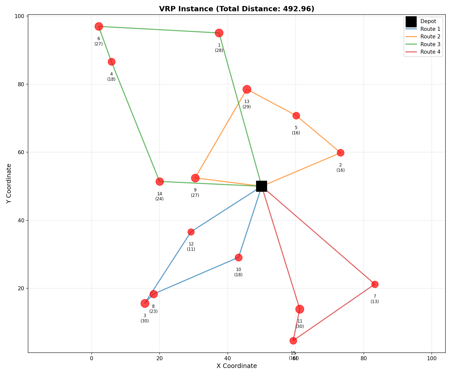
Figure 6: A sample VRP instance showing the depot and customer locations with their demands.
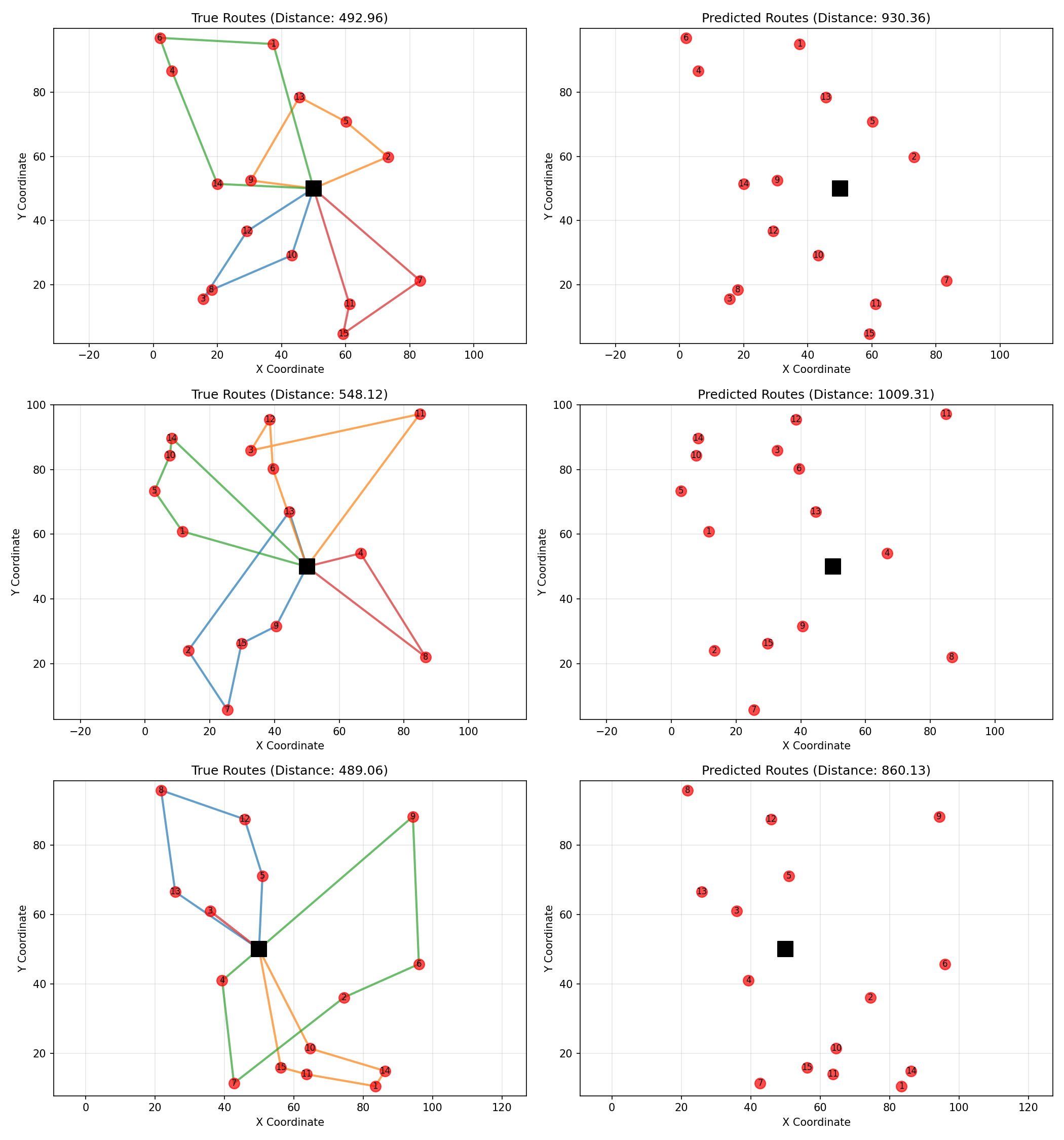
Figure 7: Side-by-side comparison of optimal routes (left) and predicted routes (right) for a VRP instance with multiple vehicles.
Complete Predicted Routes
Here's a complete visualization of predicted routes from our trained model:
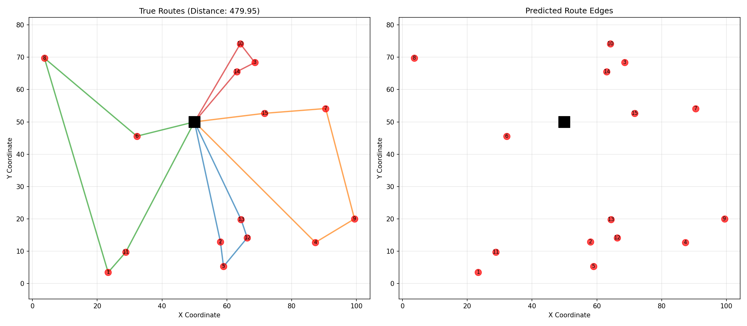
Figure 8: Complete routes constructed from the model's edge predictions. Each color represents a different vehicle route, all starting and ending at the depot.
Complete Code Repository
🔗 Graph Neural Networks Tutorial Repository
The repository includes:
- ✅ Complete VRP implementation
- ✅ TSP implementation for comparison
- ✅ Supply chain optimization
- ✅ Step-by-step tutorials
- ✅ Pre-trained models
- ✅ Visualization scripts
Conclusion
In this tutorial, you learned how to:
- ✅ Model the Vehicle Routing Problem as a graph
- ✅ Generate VRP instances with Clarke-Wright algorithm
- ✅ Design a demand-aware GNN architecture
- ✅ Handle severe class imbalance
- ✅ Extract valid routes from edge predictions
- ✅ Evaluate route quality and constraint satisfaction
Key Takeaways
| Concept | What You Learned |
| VRP | Multi-vehicle routing with capacity constraints |
| Depot | Central hub where all routes start/end |
| Demand Attention | Learn to weight nodes by demand |
| Edge Prediction | Predict route membership, not sequences |
| Class Imbalance | Only ~5-10% positive edges — use F1! |
Where to Go From Here
Improve the Model:
- Add time window constraints (VRPTW)
- Handle heterogeneous fleets
- Implement reinforcement learning
Scale Up:
- Use sparse graphs for 100+ customers
- Hierarchical clustering for large instances
- Distributed training
Deploy:
- Build an API for route optimization
- Real-time re-routing
- Integration with mapping services
🚀 Take Your Skills Further
VRP is just the beginning! The same techniques apply to:
- Pickup and Delivery: Passengers with origins and destinations
- Inventory Routing: Periodic replenishment
- Dial-a-Ride: Ride-sharing optimization
- Drone Delivery: Multi-depot, range constraints
Resources
Cover Photo by Unsplash - Logistics and Delivery
Did you find this tutorial helpful? Drop a comment below or share it with fellow ML enthusiasts!
Have questions? Feel free to leave a comment.
About the Author
Hi, I'm Israel, a data scientist and AI engineer passionate about transforming real-world challenges into innovative solutions with machine learning and data. I love mentoring and supporting others as they grow in their tech careers. When I'm not coding or coaching, you'll likely find me immersed in a game of chess or enjoying a good action movie with my family. I hope you enjoyed this blog post and learnt something.
